决策树
决策树是最经常使用的数据挖掘算法。它的重要任务就是找出数据中蕴含的信息,从数据集合中撮一系列规则,机器根据数据创建规则的过程就是机器学习的过程。
案例:测试患者要佩戴的隐形眼镜类型
使用较小的训练数据集,我们可以让算法掌握一套判断流程(决策数):眼科医生是如何判断患者要佩戴眼镜的类型的。
训练数据集中包括过往的一些诊断结果。包含患者眼部状况(散光、),医生推荐的眼镜类型(眼镜材质,是否适合隐形眼镜)等。
数据如下:
young	myope	no	reduced	no lenses
young	myope	no	normal	soft
young	myope	yes	reduced	no lenses
young	myope	yes	normal	hard
young	hyper	no	reduced	no lenses
young	hyper	no	normal	soft
young	hyper	yes	reduced	no lenses
young	hyper	yes	normal	hard
pre	myope	no	reduced	no lenses
pre	myope	no	normal	soft
pre	myope	yes	reduced	no lenses
pre	myope	yes	normal	hard
pre	hyper	no	reduced	no lenses
pre	hyper	no	normal	soft
pre	hyper	yes	reduced	no lenses
pre	hyper	yes	normal	no lenses
presbyopic	myope	no	reduced	no lenses
presbyopic	myope	no	normal	no lenses
presbyopic	myope	yes	reduced	no lenses
presbyopic	myope	yes	normal	hard
presbyopic	hyper	no	reduced	no lenses
presbyopic	hyper	no	normal	soft
presbyopic	hyper	yes	reduced	no lenses
presbyopic	hyper	yes	normal	no lenses
第一列表示患者年龄,第二列表示诊断说明,第三列表示是否有散光,第四列表示是否能够接受隐形眼镜,第五列表示最终的结果。
看似无规律的数据,我们可以通过程序进行总结,找出规律。比如:是否能接受隐形眼镜,如果 拒绝(第四列为 reduce),结果直接就为 no lenses; 如果是能接受(第四列是 normal),进一步判断是否有散光(第三列值)。如果没有散光,再判断年龄(第一列)…等等。
其实,程序是根据我们数据各个列的意义来做为判断的依据。但有个问题是:哪一列作为最优先的判断。比如上面说的,为什么要先判断是否能接受隐形眼镜?而不是先判断年龄。
程序是通过“信息增益”来进行判断的,原则就是对最终结果的影响是多少(专业术语叫:熵)。于是,我们就可以计算每一列对结果的总影响是多少。影响越大的,我们越放在前面进行判断。
用数学公式表示: l(xi)=-log2p(xi)
思路: 从数据可以看出,前四列是各项指标;最后一列是在各个指标组合下的结果。 那么,就可以先整体计算一下全体数据的熵。然后分别减去某一列,再次计算熵。两者差值越大,表示该列对结果影响越大。那么,它的判断优先度就应该越高,即:它就是决策树的第一个节点。
代码:
# -*- coding: utf-8 -*-
from math import log
import operator

decisionNode = dict(boxstyle="sawtooth", fc="0.8")
leafNode = dict(boxstyle="round4", fc="0.8")
arrow_args = dict(arrowstyle="<-")


def majorityCnt(classList):
    classCount = {}
    for vote in classList:
        if vote not in classCount.keys(): classCount[vote] = 0
        classCount[vote] += 1
    sortedClassCount = sorted(classCount.iteritems(), key=operator.itemgetter(1), reverse=True)
    return sortedClassCount[0][0]

# 划分数据集.
# dataSet: 待划分的数据集
# axis: 列数.以哪一列来划分数据集
# values: 需要返回的特征值
def splitDataSet(dataSet, axis, value):
    retDataSet = []
    # 遍历数据每一行。得到每一行的向量
    for featVec in dataSet:
        # 如果当前行向量的待划分列的值和需要返回的特征值相同,表示该行数据是我们需要的。
        # 将该列去掉(取前N列和后面的几列,重新组合成数据集)
        if featVec[axis] == value:
            reducedFeatVec = featVec[:axis]
            reducedFeatVec.extend(featVec[axis + 1:])
            retDataSet.append(reducedFeatVec)
    return retDataSet

# 计算香农值
def calcShannonEnt(dataSet):
    numEntries = len(dataSet)
    labelCounts = {}
    # 最终结果(标签)的唯一列表
    for featVec in dataSet:
        currentLabel = featVec[-1]
        if currentLabel not in labelCounts.keys(): labelCounts[currentLabel] = 0
        labelCounts[currentLabel] += 1
    shannonEnt = 0.0
    for key in labelCounts:
        prob = float(labelCounts[key]) / numEntries
        shannonEnt -= prob * log(prob, 2)
    return shannonEnt


def chooseBestFeatureToSplit(dataSet):
    # 属性(待划分数据集的依据)的个数.由于最后一列是标签,或者叫分类,就是最终的结果。所以最后一列不用计算香农值
    # 测试数据总共有 5 列,最后一列是结果。所以这里取前 4 列
    numFeatures = len(dataSet[0]) - 1
    # 整个数据集的香农值
    baseEntropy = calcShannonEnt(dataSet)
    bestInfoGain = 0.0
    bestFeature = -1

    # 遍历每一列。因为要以每一列为依据来划分数据集。然后计算每一列和结果组合的香农值。以此来判断该列对结果的影响有多大
    # 影响最大的在决策数的最顶部
    for i in range(numFeatures):
        # 找到当前列所有的值
        featList = [example[i] for example in dataSet]
        # 当前列的值去重
        uniqueVals = set(featList)
        newEntropy = 0.0
        #
        for value in uniqueVals:
            # 划分数据集.从原始数据集中去掉当前列,且只找当前列的值是遍历值的
            # 作用是为了计算每一列,每个值对最终结果的影响
            subDataSet = splitDataSet(dataSet, i, value)
            # 当前列,当前值占总数据的比例。相当于出现这种情况的概率
            prob = len(subDataSet) / float(len(dataSet))
            # 由于循环里是分别计算当前列各个值的香农植。所以将各个唯一值的香农值累加就是该列整体的香农值
            newEntropy += prob * calcShannonEnt(subDataSet)
        # 由于计算的是当前列删除后的香农值。所以该列的实际值是用总的值减去该列的总值
        infoGain = baseEntropy - newEntropy
        # 找到值最大的一列
        if (infoGain > bestInfoGain):
            bestInfoGain = infoGain
            bestFeature = i
    return bestFeature


# 创建决策树.程序会使用递归的方式来创建.每创建一层后,从数据集中去掉已经处理的列。将剩下的再进行分析。
# dataset: 数据集
# labels: 数据集每一列的含义(名称)
def createTree(dataSet, labels):
    # 取数据集最后一列的值
    classList = [example[-1] for example in dataSet]
    # 如果该列中所有的值都一样,直接返回
    if classList.count(classList[0]) == len(classList):
        return classList[0]
    # 如果当前列表只有一列
    if len(dataSet[0]) == 1:
        return majorityCnt(classList)
    # 找到对结果影响最大的一列。把它做为决策树的最顶部判断条件
    bestFeat = chooseBestFeatureToSplit(dataSet)
    # 影响最大一列的名称(自定义的)
    bestFeatLabel = labels[bestFeat]
    # 定义一个树
    myTree = {bestFeatLabel: {}}
    # 将影响最大的列从标签列表去除.后面需要将剩余的标签做进一步处理
    del (labels[bestFeat])
    # 最优列的所有值
    featValues = [example[bestFeat] for example in dataSet]
    # 最优列值去重
    uniqueVals = set(featValues)
    for value in uniqueVals:
        # 复制 labels ,然后使用,以免对原数据造成影响
        subLabels = labels[:]
        # 递归调用本方法。传入的数据集是去掉当前最优列的集合。意思是从剩余的列中再找最优列,然后再处理。
        # 通过调归方法,可以依次找到对结果影响最大的列
        myTree[bestFeatLabel][value] = createTree(splitDataSet(dataSet, bestFeat, value), subLabels)
    # 树的各个判断条件就是各列的名字。最终终止点就是数据集的最后一列对应的值。判断条件的值就是该列的值。
    return myTree

fr = open('lenses.txt')
lenses = [inst.strip().split('\t') for inst in fr.readlines()]
# 数据每一列的含义
lenseslabels = ['age', 'prescript', 'astigmatic', 'tearRate']
lenesTree = createTree(lenses, lenseslabels)
print lenesTree
输出的结果是:
{'tearRate': {'reduced': 'no lenses', 'normal': {'astigmatic': {'yes': {'prescript': {'hyper': {'age': {'pre': 'no lenses', 'presbyopic': 'no lenses', 'young': 'hard'}}, 'myope': 'hard'}}, 'no': {'age': {'pre': 'soft', 'presbyopic': {'prescript': {'hyper': 'soft', 'myope': 'no lenses'}}, 'young': 'soft'}}}}}}
从结果可以看出判断的顺序:先判断 tearRate,如果是 reduced,直接返回 no lenses; 如果是 normal,进入下一步 astigmatic 的判断:如果是 yes,进一步判断 prescript…
我们把这串 json 格式格式化后会稍微清晰一点。当然,我们可以生成图片类似流程图,那就更直观了:
def getNumLeafs(myTree):
    numLeafs = 0
    firstStr = myTree.keys()[0]
    secondDict = myTree[firstStr]
    for key in secondDict.keys():
        if type(secondDict[key]).__name__=='dict':#test to see if the nodes are dictonaires, if not they are leaf nodes
            numLeafs += getNumLeafs(secondDict[key])
        else:   numLeafs += 1
    return numLeafs

def getTreeDepth(myTree):
    maxDepth = 0
    firstStr = myTree.keys()[0]
    secondDict = myTree[firstStr]
    for key in secondDict.keys():
        if type(secondDict[key]).__name__=='dict':#test to see if the nodes are dictonaires, if not they are leaf nodes
            thisDepth = 1 + getTreeDepth(secondDict[key])
        else:   thisDepth = 1
        if thisDepth > maxDepth: maxDepth = thisDepth
    return maxDepth

def plotNode(nodeTxt, centerPt, parentPt, nodeType):
    createPlot.ax1.annotate(nodeTxt, xy=parentPt,  xycoords='axes fraction',
             xytext=centerPt, textcoords='axes fraction',
             va="center", ha="center", bbox=nodeType, arrowprops=arrow_args )

def plotMidText(cntrPt, parentPt, txtString):
    xMid = (parentPt[0]-cntrPt[0])/2.0 + cntrPt[0]
    yMid = (parentPt[1]-cntrPt[1])/2.0 + cntrPt[1]
    createPlot.ax1.text(xMid, yMid, txtString, va="center", ha="center", rotation=30)

def plotTree(myTree, parentPt, nodeTxt):#if the first key tells you what feat was split on
    numLeafs = getNumLeafs(myTree)  #this determines the x width of this tree
    depth = getTreeDepth(myTree)
    firstStr = myTree.keys()[0]     #the text label for this node should be this
    cntrPt = (plotTree.xOff + (1.0 + float(numLeafs))/2.0/plotTree.totalW, plotTree.yOff)
    plotMidText(cntrPt, parentPt, nodeTxt)
    plotNode(firstStr, cntrPt, parentPt, decisionNode)
    secondDict = myTree[firstStr]
    plotTree.yOff = plotTree.yOff - 1.0/plotTree.totalD
    for key in secondDict.keys():
        if type(secondDict[key]).__name__=='dict':#test to see if the nodes are dictonaires, if not they are leaf nodes
            plotTree(secondDict[key],cntrPt,str(key))        #recursion
        else:   #it's a leaf node print the leaf node
            plotTree.xOff = plotTree.xOff + 1.0/plotTree.totalW
            plotNode(secondDict[key], (plotTree.xOff, plotTree.yOff), cntrPt, leafNode)
            plotMidText((plotTree.xOff, plotTree.yOff), cntrPt, str(key))
    plotTree.yOff = plotTree.yOff + 1.0/plotTree.totalD

def createPlot(inTree):
    fig = plt.figure(1, facecolor='white')
    fig.clf()
    axprops = dict(xticks=[], yticks=[])
    createPlot.ax1 = plt.subplot(111, frameon=False, **axprops)    #no ticks
    #createPlot.ax1 = plt.subplot(111, frameon=False) #ticks for demo puropses
    plotTree.totalW = float(getNumLeafs(inTree))
    plotTree.totalD = float(getTreeDepth(inTree))
    plotTree.xOff = -0.5/plotTree.totalW; plotTree.yOff = 1.0;
    plotTree(inTree, (0.5,1.0), '')
    plt.show()

# 加上前面生成树的相关代码
createPlot(lenesTree)
生成的图如下:
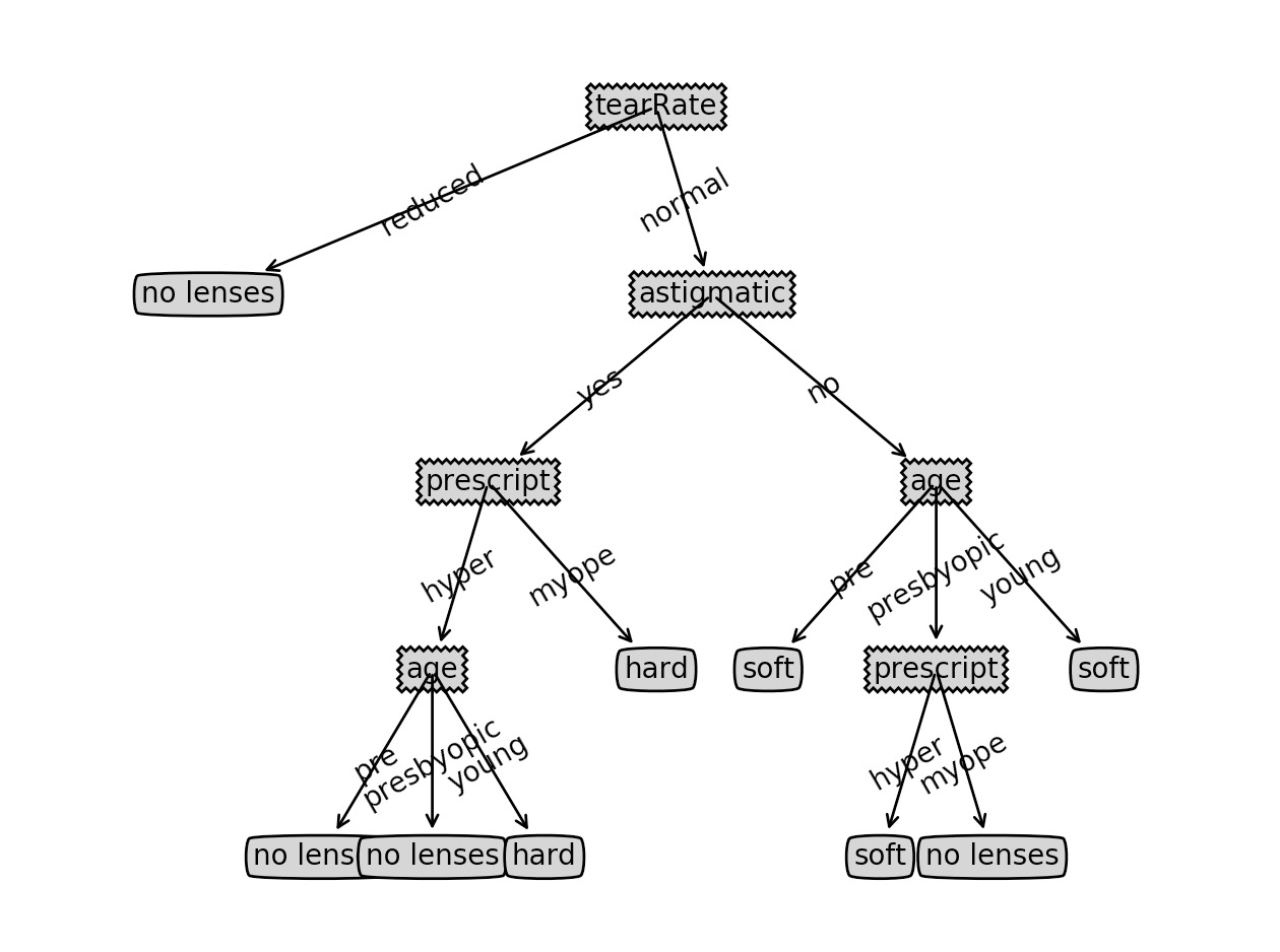
有了这个决策的逻辑,我们就可以对某种情况进行推断。比如现在有一位新患者,通过调查,我们知道他对各个判断指标的数值,那么我们就可以按上述判断逻辑走一遍,然后推算出他可能的结果。